
When debugging network quality, we typically focus on two factors: latency and throughput (bandwidth). Latency is relatively easy to verify by simply pinging or performing a traceroute to gain insights. This article shares a method for debugging throughput, with a focus on TCP congestion control.
Scenarios that prioritize throughput are usually what are known as Long Fat Networks (LFN). For instance, downloading large files. If throughput hasn’t reached the network’s limit, it may be primarily affected by three factors:
Bottlenecks at the sending end typically involve insufficient buffer size, as the sending process involves the application calling a syscall to place data in the buffer, then having the system send it out. If the buffer is full, the application will block (assuming a blocking API is used) until the buffer becomes available and can continue to write, following the producer-consumer model.
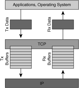
Bottlenecks at the sender are generally easier to debug; often, you can simply check application logs to see when blocks occurred. In most cases, it’s the second or third situation, which are more challenging to diagnose. This happens when the application’s data has been written to the system’s buffer, but the system hasn’t sent it out quickly enough.
TCP, to optimize transmission efficiency (note that this refers to overall network efficiency rather than just one TCP connection), will:
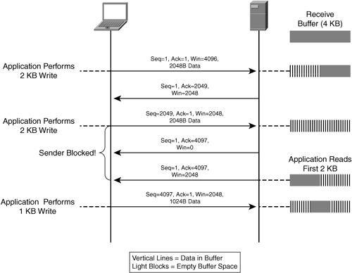
To protect the receiver, when connections are established at both ends, they agree on the receiver’s buffer size (receiver window size, rwnd), and during subsequent sends, the receiver also reports its remaining window size in every acknowledgment packet. This ensures the sender doesn’t exceed the receiver’s buffer size. (Meaning that the sender is responsible for ensuring the total unacknowledged doesn’t exceed the receiver’s buffer.)
To protect the network, the principle is also to maintain a window, called the Congestion Window (cwnd), which is the current network limit. The sender won’t transmit more data than this window’s capacity (the total unacknowledged won’t exceed cwnd).
How do we find this cwnd value?
This is crucial—by default, the algorithm is cubic, but other algorithms like Google’s BBR can be used.
The main logic is slow start: send data to test; if the receiver’s acknowledgment is correctly received, it indicates the network can handle this throughput. Then cwnd is doubled, and testing continues until one of the following conditions occurs:
Point 2 is easy to understand, indicating that network throughput isn’t a bottleneck; the bottleneck is at the receiver’s insufficient buffer size. cwnd can’t exceed rwnd, or the receiver will be overloaded.
For point 1, essentially, the sender uses packet loss to detect network conditions. If no packet loss occurs, everything is normal. If packet loss occurs, the network can’t handle this sending speed, and the sender will halve the cwnd.
But the real reason for point 1 may not be a network throughput bottleneck; it might be the following situations:
Reasons 2 and 3 can both cause a drop in cwnd, preventing full utilization of network throughput.
The above is the basic principle, and now let’s introduce how to pinpoint such issues.
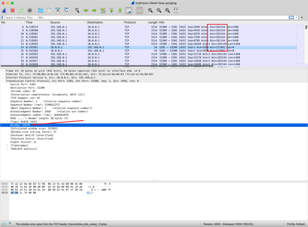
This window size is directly in the TCP header, so you just need to capture it to see this field.
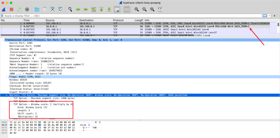
However, the actual window size needs to be multiplied by a factor, which is in the TCP options. Thus, to analyze a TCP connection’s window size, you must capture packets during the handshake phase, or else the negotiated factor cannot be known.
Congestion control is a dynamic variable calculated by the sender through algorithms, and it won’t be reflected in the protocol’s transmitted data. Therefore, to observe it, you must look at the sending machine.
In Linux, you can use certain options to print out the parameters of a TCP connection.
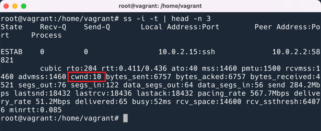
This showcases units as real size 1460 bytes * 10.
Wireshark offers highly useful statistical features that allow you to immediately identify where the current bottleneck occurs. However, when I first opened this graph, I was clueless and couldn’t find resources on how to interpret it. Fortunately, I learned, and I document it here to teach you as well.
First, the opening method is as follows:
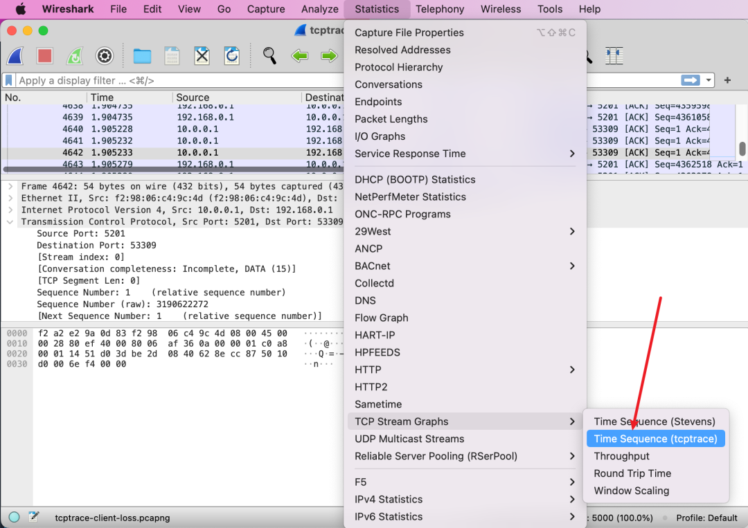
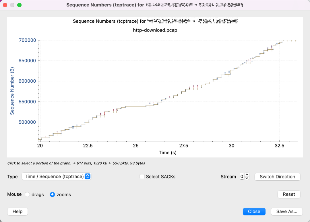
Then you will see a graph like this.
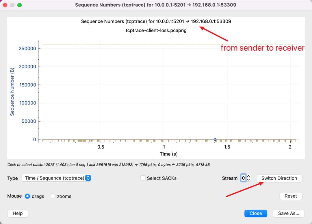
It’s crucial to know that the tcptrace graph represents single-direction data transmission, as TCP is a duplex protocol, meaning both ends can send data. At the top, it shows the current graph data is from 10.0.0.1 to 192.168.0.1. You can switch the view’s direction by clicking the button at the bottom right.
The X-axis represents time, which is easy to grasp.
Understanding the Y-axis, which represents the Sequence Number in the TCP packets, is critical. All data in the diagram is based on this Sequence Number.
So, if you see a chart as above, it indicates you’re viewing it backward because the Sequence Number hasn’t increased, meaning there’s almost no data transmission. You need to click Switch Direction.
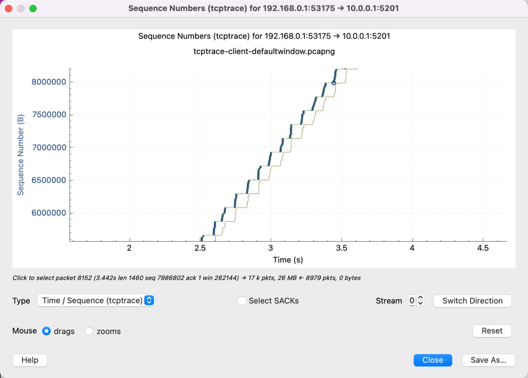
That’s more like it; you can see our transmitted Sequence Number increases over time.
There are three lines here with the following meanings:

In addition, there are two other types of lines:
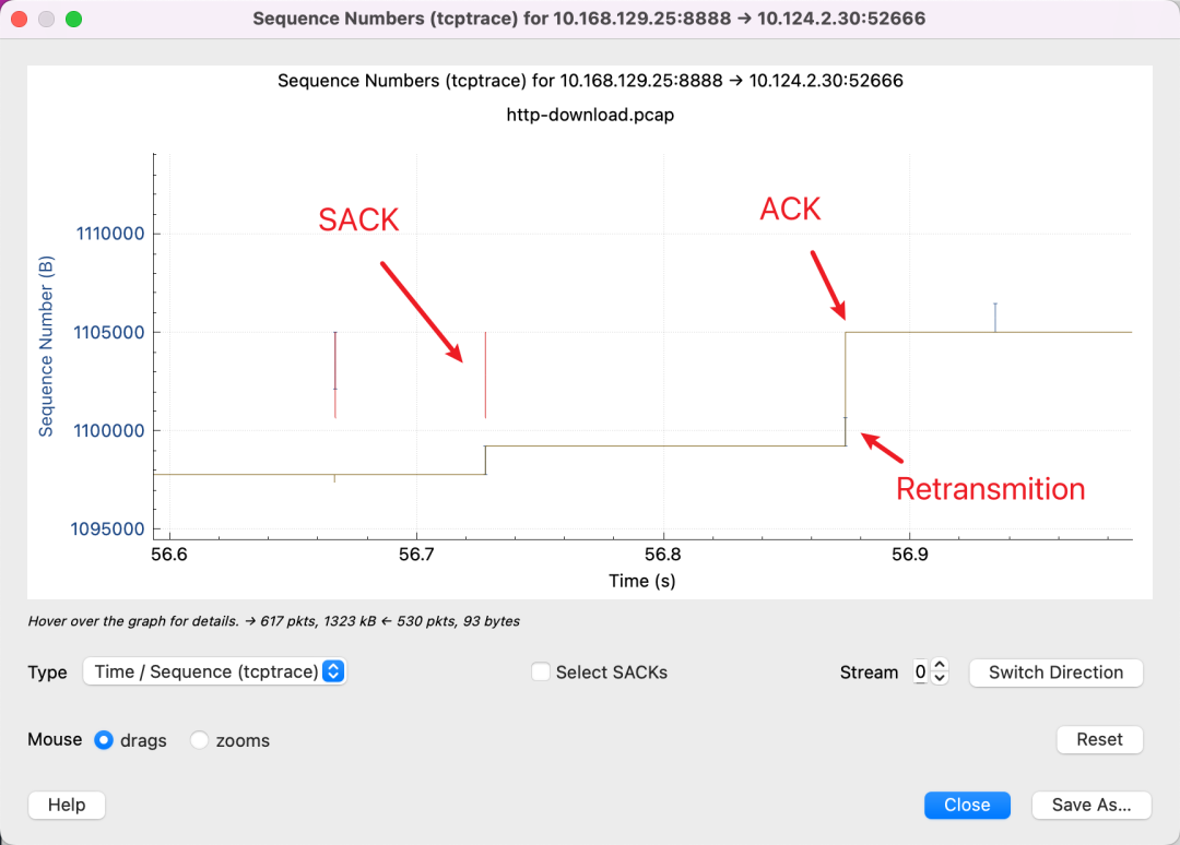
Always remember that the Y-axis represents the Sequence Number. The red line indicates the SACK line showing the segment of Sequence Number that has been received. Coupled with the yellow line showing ACKed Sequence Number, the sender will know there’s a missing packet in the blank space between the red and yellow lines. Therefore, retransmission is required. The blue line indicates that retransmission has occurred.
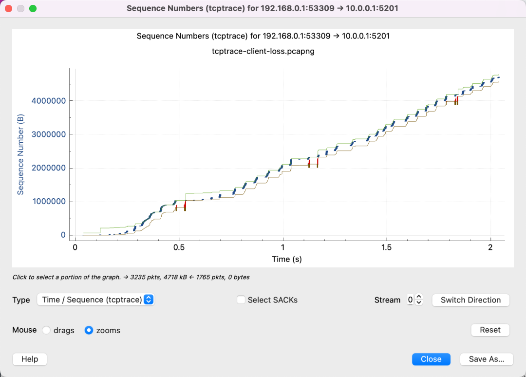
Understanding how to interpret these graphs allows us to recognize several common patterns:
Many red SACKs indicate the receiver repeatedly states: “I didn’t receive a packet,” or “I missed a packet.”
This graph shows that as soon as the yellow line (receiver’s ACK) rises, the blue follows (sender starts sending) until it fills the green line (window size), indicating the network isn’t a bottleneck and suggests increasing the receiver’s buffer size.

This chart shows that the receiver’s window size is far from a bottleneck, with plenty of available space.
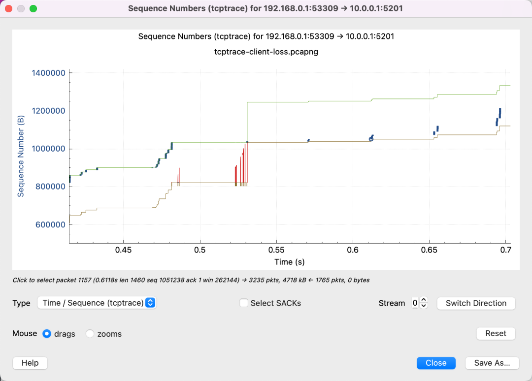
Upon magnification, it shows many packet losses and retransmissions, sending only small amounts of data each time. This suggests the cwnd might be too small, constrained by congestion control algorithms.
[1]
mtr:
[2]
rfc7323:
[3]
BBR:
[4]
TCP handshake node negotiation through TCP Options:
[5]
TCP MSS.
[6]
Colleague: